At this point you should have R and R Studio installed on your computer, if that is not the case check out Getting Started with Data Science (Part I) in this series.

A brief primer on R

As with Python, R is a interpreted language , where they differ though is that Python is a general purpose language that can be used for many different applications. R is a statistical computing language designs for data analysis and graphical representation of data. You are not going to go out and design a video game using R, its main purpose in life is to analyze data.

The beauty of R is, like Python, it is very easy to work with and fairly straightforward to read and write. A huge benefit is R’s IDE, R Studio, in my opinion this is one of the best IDEs out there, it allows the user to execute each line or block of code as it is written and see the progress of how the script (what a R program is called) is progressing data. R came about in 1991 and the first stable release was in 2000.

A simple program in R

To get started writing code in R first we need to open up R Studio, once open you will see three separate viewports, as we use the items within these viewports we will discuss what they are and do.

To get up and running wirting in R we will need to create an R script, in the upper left hand corner of R Studio there is an icon with a green + symbol, clicking that will bring up a context menu to choose the type of file you’d like to create, for this exercise we will select R Script.

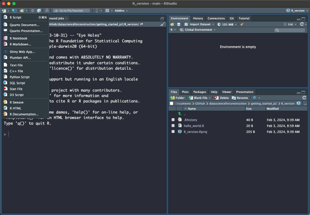
Now you will have a fourth viewport which is in the upper left hand quadrant of the window. This is you R Script and where you will start writing you code.

Writing our first script

Inside the R Script you have just created write the following code.

print("hello world")

Now comes one of the beauties of R and R Studio, while still on the line containing print("hello world")hit ctrl+enter or cmd+return and in the terminal in the lower left hand viewport you will see the output in the terminal. This alows us to see the output of the code as it is being written in the IDE, similar to notebooks which we will cover in a separate article.

Diving deeper

Since R is not a general purpose language such as Python we are not going to create the same program we did in the Part II where we discussed the basics of python. Instead we are going to handle some data and perform some basic manipulations and visualizations.

Create a new R Script titled whatever you’d like. The primary tools used for construction data handling being Excel we will create some simple data and use R to go through that data similar to how we would use Excel. In your new script write the following lines of code.

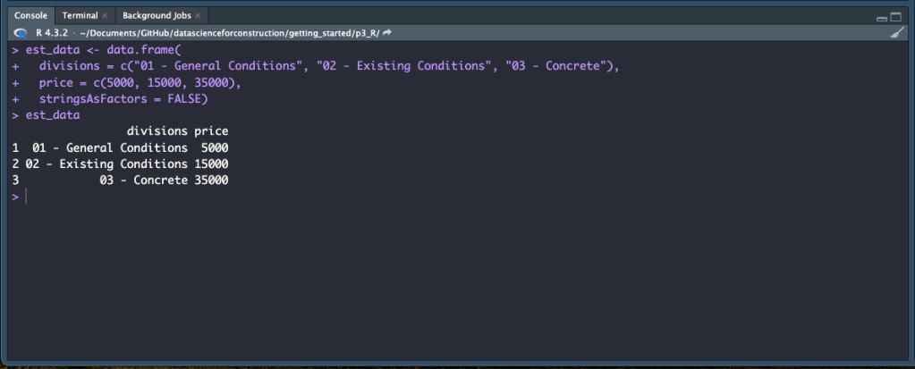
est_data <- data.frame(
  divisions = c("01 - General Conditions", "02 - Existing Conditions", "03 - Concrete"),
  price = c(5000, 15000, 35000),
  stringsAsFactors = FALSE)
est_data

The first thing we are doing is creating a dataframe, think of dataframes as a basic spreadsheet with rows and columns, here we are naming our dataframe est_data. The <- in R is the the same as = in python, in fact you can use = if you’d like but <- is the R way. We use the data.frame() function to create a new dataframe and inside the fuction we use the c() function to concatenate the values we are using to create the dataframe. We create a column called divisions, then we assign it the values 01 – General Conditions, 02 – Existing Conditions, 03 – Concrete. Then we create a price column with values using the same method. Finally we set stringsAsFactors to FALSE. We wont worry at this time about what stringsAsFactors does or is for now we will set it to false. Again with R after you write each line or block hit ctrl+enter or cmd+return to run the code and the results will populate in the terminal. You will see here that we now have a dataframe in the terminal with the data we entered.

Next we may want to add some new data or manipulate the data we have. Write the following code after the code from the previous section.

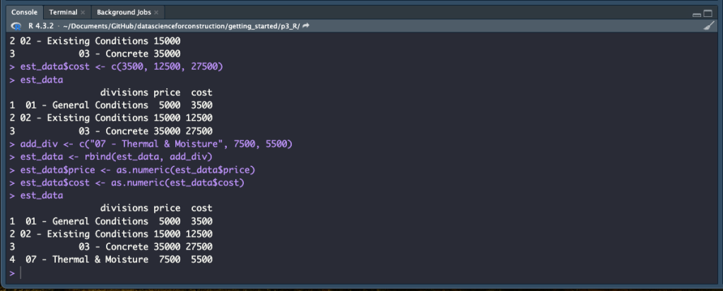
est_data$cost <- c(3500, 12500, 27500)
est_data

Here we are adding a column to our dataframe. We state the dataframe we are using with est_data, then we add $cost after to give a name to a new column. We then pass the values to that column again using the c() function and call the dataframe est_data to view our results.

Now let’s say we want to add a column to the dataframe, write the following code after the code we wrote in a previous section.

add_div <- c("07 - Thermal & Moisture", 7500, 5500)
est_data <- rbind(est_data, add_div)
est_data$price <- as.numeric(est_data$price)
est_data$cost <- as.numeric(est_data$cost)
est_data

Here we have created a variable titled add_div and assigned it a vector with values for all three columns using the c() function. We then bound the vector to the dataframe using the rbind() function. Next with the est_datat $price and est_data$cost columns we are casting the data to a numeric type and we again call the dataframe to see the results.

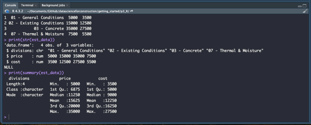
At this point we may want to check our data and the structure and summary of our dataframe. Enter the following lines and after each hit ctrl+enter or cmd+return.

print(str(est_data))
print(summary(est_data))

The str() function shows the internal structure of the dataframe and the summary() function show the summary statistics of the dataframe. Both can be used to check the data, validate the data types, and see the summary statistics.

Let’s add a new column and populate it with the result of a basic mathematic formula. Write the following code after the code from the previous section.

est_data$margin <- ((est_data$price - est_data$cost) / est_data$price) * 100
est_data

Here we are creating a new column called margin using est_data$margin and assigning it a value using ((est_data$price - est_data$cost) / est_data$price) * 100. This takes the price less the cost and divides it by the price to get the decimal for the margin and then multiplies this by 100 to get the percentage margin. Run each line once written to execute the code and see the results.

Data manipulation with loops

Now we may want to add a couple of columns to see the outcome of a lowering or raising the cost by a certain percentage. Write the following code next.

for(i in c(-5, 10)) {
  est_data[, paste0("cost_", i, "%_change")] = 
    est_data$cost * (1+i/100)
  est_data[, paste0(i,"%_margin")] = 
    ((est_data$price - (est_data$cost * (1+i/100))) / est_data$price) * 100
}
est_data

The first statement we make is the for(i in c(-5,10)){}, the statement in the () is our argument or condition which in this case is for the amount of items “i” in the vector [-5, 10], made using the c() function. Inside {} we call the est_data dataframe, when we perform function on dataframe we use [] and inside the [] we have [rows, columns]. inside our dataframe we are using the paste0() function which concatenates characters into vectors, in this case we have “cost_” then i (which here is -5 and 10), then “%_change”. We are assigning this new column a value based on multiplying the value in the cost column by 1 plus i (-5, 10) divided by 100. The next line is following the same procedure we are creating a column and then assigning it a value using the same margin calculation we used earlier. Since this is a loop, the process we outlined works its way through the dataframe row by row, column by column and applies the statement we outlined.

Now that we have created a dataframe, added some columns and rows and manipulated the data by performing some calculations we want to see the totals of some of the different columns. To do this write the following code.

ttl_cost <-sum(est_data$cost)
ttl_5_cost <- sum(est_data$`cost_-5%_change`)
ttl_10_cost <- sum(est_data$`cost_10%_change`)

cat(ttl_5_cost, ttl_cost, ttl_10_cost)

In the preceding code we are assigning variables such as ttl_cost and assigning them values based on the sum of the data in a given column such as est_data$cost. To show these results in one line in the terminal we use the cat() function and include the variables in the function.

Creating functions in R

Similar to the number converter we created in Python in part II, we can use R to run a set of calculations to perform some geometry that we may want to do quickly form time to time. To be able to use the same math over and over with different parameters we need to create a function. To create a function in R you name it, give it a set of parameter names, and give it a set of instructions to execute. You can continue writing the following in the same Script or you could create a new script for this.

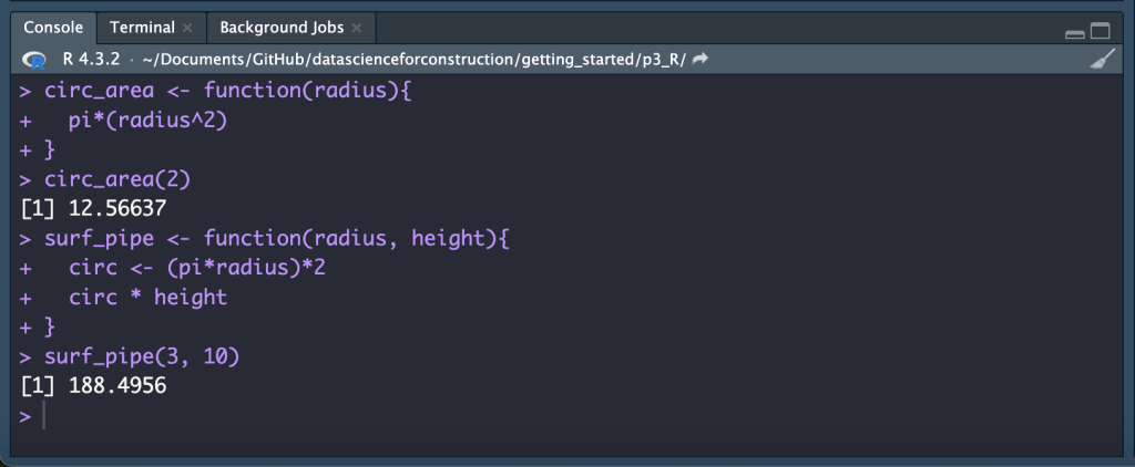
circ_area <- function(radius){
  pi*(radius^2)
}

circ_area(2)

The above function executes a set of instructions to calculate the area of a circle using the parameter of radius. We first name our formula circ_area and make it a function <- function(){}, inside the () we state our parameters for this function our parameter is radius, inside the {} we stated the instructions to execute when the function is run, for this case we use 𝜋r² which we notate in our code as pi*(radius^2). Once the function is written we use ctrl+enter or cmd+return to execute the code and create the function, now we can call the function and pass it a parameter like this circ_area(2) here we are stating we have a circle with a radius of 2 and we are using our function to calculate the area which R returns in the terminal as 12.56637.

We created a function to find the area of a circle, lets create one to find the surface area of a pipe, this requires that we have two parameters. Write the following code.

surf_pipe <- function(radius, height){
  circ <- (pi*radius)*2
  circ * height
}

surf_pipe(3, 10)

As in the last example we created a function by naming it surf_pipe in this case and assigning it as a function using <- function(){}. For us to calculate the surface area of a pipe we need to know the radius of the pipe and the length of the pip so we need to include two parameters in our function, function(radius, height), since length is a base function in R we use height as our parameter name. Next we write the instructions by creating a variable called circ and assigning it a value using (pi*radius)*2 to get the circumference of the circle. We then use our variable circ and multiply it by our parameter height. We create the fucntion, and then called the function with parameters of a radius of 3 and height of 10 using surf_pipe(3, 10) which yields the result of 188.4956.

Last we will create one more function using more parameters and more calculation. We wnat to determine the surface area of a steel beam, we know the thickness of the metal the web and flange dimensions, and the length. Write the following code.

surf_beam <- function(flange, web, thickness, long) {
  ttl_flange <- (flange * 2) + ((flange - thickness) * 2)
  ttl_web <- web * 2
  edge <- thickness * 4
  ttl_perim <- ttl_flange + ttl_web + edge
  ttl_perim * long
}

surf_beam(8, 4, 0.5, 10)

As in the last two examples we name our function and using function(){} we give it parameters and a set of instructions. For this examples we need to create several variables to calculated the total flange, total web, and edge dimensions so we can calculate the total perimeter, from there we can multiply the perimeter by the length (here we use long as our parameter as length is a base function in R). We create the function hitting ctrl+enter or cmd+return and call the function with surf_beam(8, 4, 0.5, 10) and the result is 410.

Conclusion

Congratulations, you have take first steps in working with data in R, you created vectors, dataframes, wrote loops, used and created functions. R is a great language for data exploration, analysis, and statistical computing, there is a major benefit is using both Python and R when working with data, for some tasks one may be more suited than the other, but having a good basic foundation of both will help you decide what to use when. I highly encourage you to continue learning about R through both digital and print resources of which there are many.

Resources

The code used in this article can be found in the companion repository by clicking the button below.