Introduction

If you are already familiarity with FRED and use it feel free to skip this short introduction. FRED, stands for Federal Reserve Economic Data, it is an online repository of economic data that is gathered from multiple sources. There approximately 823,000 time series from 114 sources. You can explore the FRED database at https://fred.stlouisfed.org/.

Finding the data

Before we can explore data from FRED we need to find the data set we want to explore, this can be a bit tricky. When you arrive at the FRED site, you can search for the data in the search bar, you can select to search by trending terms, or the data by category, release, source, tag, or release calendar.

Using the API

First off what is an API, application programming interface, in very simple terms, it is a way for us to request information from another software, in this case a database managed by FRED, and get a response back. Based on the criteria we use in our request, we define what we want, and how we want it, within the constraints set by the responding party.

We will explore two methods on requesting data, receiving a response, and processing this data to be visualized. Then we will pull in multiple datasets and visualize them side by side.

The basics

To get started using the FRED API we need to request an API key so that the system knows who we are and that we have authorization to request data. To do this go to https://fred.stlouisfed.org/docs/api/api_key.html, here you can set up an account and request an API key, it will be a 32 character lowercased alpha numeric string. While you are on the site, explore the API documentation, its not necessary to know it all or even review it but it may help understand a bit more about the API and how requests are processed.

To get started we need to install/import some libraries we will use in the following code, enter the following lines, if using a notebook like Jupyter/Colab I keep the pip install in the first cell and the remainder in the following as fredapi is not included in the colab standard libraries. Note: if you are using colab you will need to use !pip if you are coding this in Jupyter or in a script just use pip.

!pip install fredapi

from datetime import date
from fredapi import Fred
import json
import requests
import numpy as np
import pandas as pd
import matplotlib.pyplot as plt

Next we want to create a global variable, here we titled it FRED_API_KEY, you will assign this variable your API key provided by FRED.

FRED_API_KEY = 'enter your api key here'

Since we are exploring data, one of the best ways to do this is to visualize the data. We want to create to functions that we can use later to visualize the data. Write the code in the next two cells.

def data_plot_m1(series, label):
  series.plot(color='cyan', style='-')
  plt.xlabel('Time')
  plt.ylabel('Value')
  plt.title('Time Series')
  plt.legend([label])
  plt.show()

In this first function we create a function and give it two parameters, series and label. Using the dot (.) operator we use the matplotlib plot function to plot the series, we then give the plot a color and style. We assign an X & Y axis label, a title, and using the label parameter a legend. We then use the show function to print the graph.

def data_plot_m2(df, label):
  plt.plot(df.date, df.value)

In the second function we are plotting a data frame and not a series, we create our function and assign to parameters df and label, we then use the plot function and pass the X & Y values called date and value into the function.

Method 1: Using the fredapi library

For method one, we will be using the fredapi library to retrieve data from FRED. Write the following block of code.

fred = Fred(api_key=FRED_API_KEY)
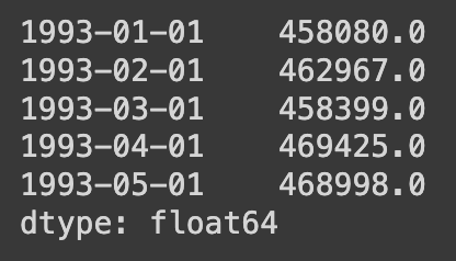
fred_data_m1 = fred.get_series('TTLCONS')
fred_data_m1.head()

Here we create a variable called fred and using the Fred function and the api_key parameter we pass our global variable for our API key. We then create a variable for our series and using the fred.get_series function we use the name of the series we want (TTLCONS) to retreive the data. We then use the pandas .head() function to view the first five rows of data. The image below is what the .head() function will return.

We now use the plotting fucntion for method one we created earlier, we pass in our series we pulled from FRED and give it a title. Write the following code.

data_plot_m1(fred_data_m1, 'Total Const Spending')

The image below is the graph that the function (data_plot()) will return.

Method 2: Using the API and requests library

The second method we can use to retreive data from FRED is by using the requests library and the API url with parameters for the data we want. This method is a bit more intensive but also allows for a bit more flexibility. The following code will create a variable with the FRED API url. We then create a dictionary called parameters, a dictionary in python alows use to store data with both a key and a value, in the dictionary below ‘series_id’ is a key and ‘TTLCONS’ is the value, these keys and values are separated by a colon “:”, and each pair is separated by a coma, We tell python we are making a dictionary by writing the data inside {} (curly braces).

api_url = 'https://api.stlouisfed.org/fred/series/observations'

parameters = {'api_key': FRED_API_KEY,
              'series_id': 'TTLCONS',
              'observation_start': '2013-01-01',
              'observation_end': '2022-01-01',
              'file_type': 'json',
              }

Next we need to combine the base url with our parameters in a way consistant with the FRED API documentation. We create a new variable called request_url we assign this the api_url (which is the base url) then we add ‘?’ (this is the first character needed after the base url), then we join the ‘&’ symbol with each of the parameters. To do this we run a loop inside of the join function. We start this by stating that k (key) equals v (value), so that it prints each key and value in the dictionary with ‘=’ in between them, then we loop over each pair in the dictionary (for k, v in parameters.items()). This loop takes each parameter (key=value) and adds & in front of it and appends it to the base url.

request_url = api_url + '?' + '&'.join([f'{k}={v}' for k, v in parameters.items()])

The output of this code is the following url, https://api.stlouisfed.org/fred/series/observations?api_key=your_api_key_here&series_id=TTLCONS&observation_start=2013-01-01&observation_end=2022-01-01&file_type=json, this is the url we send to the FRED API to request the data we want.

Next we want to request the data, using the request.get() function we give the url as the parameter and assign it to a new variable called response. The line response.raise_for_status() will give you an error code if the url or data format is incorrect or if the data does not exist.

response = requests.get(request_url)
response.raise_for_status()

fred_api_data = response.json()
print(fred_api_data)

The image below is what the print functino will reutrn of the json returned by the above code.

We then need to normalize the json, as the current format is one long line, we normalize using the pandas json_normalize() function and we state that we want to normalize on the observations, this will remove the first section of data which is just the parameters we requested.

fred_data_m2 = pd.json_normalize(fred_api_data['observations'])

fred_data_m2.head()

Using the pandas head function we can now see the first five rows of our data frame and the format and data included.

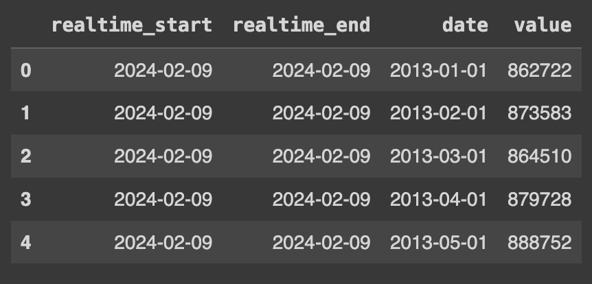
For our usage we do not need the two columns for realtime start and end, we just want the date and value columns. We use the pandas drop() function and the dot (.) operator to pass the data frame to the drop function and then state the columns we want to drop. [[0,1]] are the indices for the first two columns, pandas data frames start with index 0 for both rows and columns, and axis=1 is the columns axis, while axis=0 would be the row axis. We again use the head() function to veiw the first five rows of data.

fred_data_m2.drop(fred_data_m2.columns[[0,1]], axis=1, inplace=True)

fred_data_m2.head()

At this stage we want to look at the underlying data types of the data frame. We need to know what the data types are as when we go to plot the data we will need the date column to be in a date format and the value columns to be in a numerical format. When we run the code below we see that both our data types are object and are not date or numbers.

fred_data_m2.dtypes

Lets create a dictionary with our column names as the key and the data type as the value. We can pass this dictionary to the .astype() function to convert our objects to a date time format for the date column and a float for the value. run the .dtypes method on the data frame again to check the results.

type_convert = {'date': np.datetime64,
                'value': float}

fred_data_m2 = fred_data_m2.astype(type_convert)

fred_data_m2.dtypes

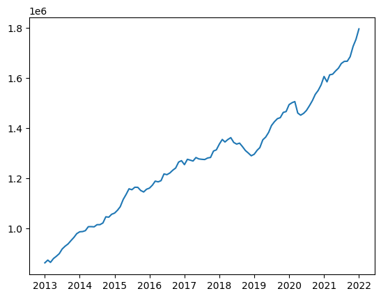
Now that our data frame is in the right format and right data types we can use our plotting function from earlier to plot the data.

data_plot_m2(fred_data_m2, "ttl const spend")

Working with Multiple Datasets

Often we don’t necessarily want to just look at one data set, we may want to look at multiple and plotting them side by side to explore how or if they are interrelated before we process and explore the data future. To do this we will use method 2 to gather, process, and visualize several data sets from FRED.

To get started we will create three sets of our parameters, one for each dataset we want to explore.

api_url = 'https://api.stlouisfed.org/fred/series/observations'

ttl_cons = {'api_key': FRED_API_KEY,
            'series_id': 'TTLCONS',
            'observation_start': '2003-01-01',
            'observation_end': '2023-01-01',
            'file_type': 'json',
            }

ttl_non_res = {'api_key': FRED_API_KEY,
              'series_id': 'TLNRESCONS',
              'observation_start': '2003-01-01',
              'observation_end': '2023-01-01',
              'file_type': 'json',
              }

ttl_res = {'api_key': FRED_API_KEY,
           'series_id': 'TLRESCONS',
           'observation_start': '2003-01-01',
           'observation_end': '2023-01-01',
           'file_type': 'json',
           }

Since we are processing more than one set of data we will create a function to process the incoming data from FRED. We use the same code for the api request and response, normalizing the JSON, creating the conversion dictionary, converting the data types, and renaming the columns. We then pass the parameters into the function to create our three data frames.

def get_fred(parameters, name):
  request_url = api_url + '?' + '&'.join([f'{k}={v}' for k, v in parameters.items()])

  response = requests.get(request_url)
  response.raise_for_status()
  fred_api_data = response.json()

  df = pd.json_normalize(fred_api_data['observations'])
  df.drop(df.columns[[0,1]], axis=1, inplace=True)
  type_convert = {'date': np.datetime64,
                'value': float}
  df = df.astype(type_convert)
  df.rename(columns = {'value' : name}, inplace = True)

  return(df)

res = get_fred(ttl_res, 'res')
non_res = get_fred(ttl_non_res, 'nres')
cons = get_fred(ttl_cons, 'cons')

At this point we have three data frames and we really only need or want one to visualize the data, so we need to merge them together. We create a new data frame called subgroups and using the .merge() method on the “res” data frame we pass in the “non_res” data frame, we use the on=’date’ argument to state that the data frames share the date column, and we use the how=’outer’ argument to state that we want to include all rows wether both data frames have data in them or not. Then we will repeat the process by creating a new “all_data” data frame using our new “subgroups” data frame and the .merge() function to add in the “cons” data frame. Printing this we can see that we have one date column and three value columns all with the names of the data frames we merged in.

subgroups = res.merge(non_res, on='date', how='outer')
all_data = subgroups.merge(cons, on='date', how='outer')
all_data.head()

And finally we will plot this data to see all the data in the same plot. We create three plots and use the date column as the x axis and the values of each data set as the y values. We label each, label the X and Y axis, and bring in a legend.

plt.plot(all_data['date'], all_data['res'], label='Residential')
plt.plot(all_data['date'], all_data['nres'], label='Non-Residential')
plt.plot(all_data['date'], all_data['cons'], label='Total')
plt.xlabel('Date')
plt.ylabel('Spending')
plt.title('Total, Residential, and Non-Residential Construction Spending')
_ = plt.legend()

Conclusion

With the large amount of data included in the FRED library there is a huge amount of possibilities to explore and a great deal of analysis to be done. Spend some time on the FRED site looking at different data sets, exploring how detailed or how broad some of the data is. You can always download the data in csv or excel format and look at the data before you bring it into python for analysis. If you want to just explore the data in Excel there is an Excel add-in as well that will pull in different data sets directly into Excel which we will cover in a separate article.

Resources

The code used in this article can be found in the companion repository by clicking the button below.