Introduction

We have an upcoming project and the questions is asked whats the cash demand for the project. We want to show the cash needed to perform each given part or phase of the project, over the duration of those parts or tasks, and show the total project demand and the monetary resources needed. We have an estimate prepared for the project and a schedule. Let’s get started.

Preparing the Data

First we want to make sure our estimate and schedule are in a table that we can reference with our equations. A sample set of data and everything covered in this article can be found below in the repository.

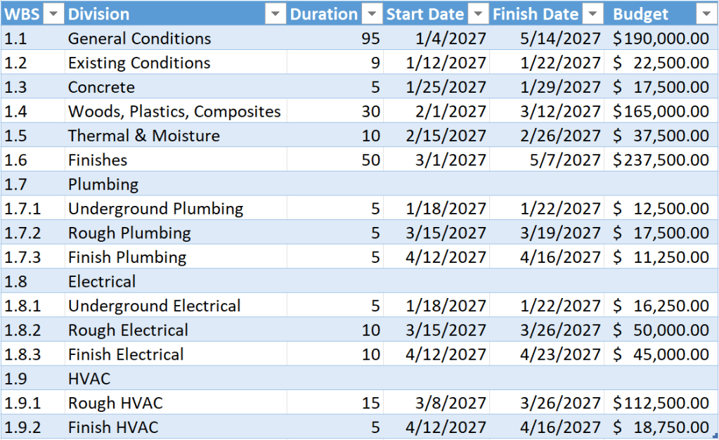
For this example we are using our divisions as our estimate and schedule sections. We have each division and our total cost per division (not the price, the cost) and we have the start and finish dates for those divisions.

Setting Up

In our reference table we need to get the cost per day, we add a new column and in that column we will add the following formula

=IF(ISBLANK([@Duration]), "", [@Budget]/[@Duration])

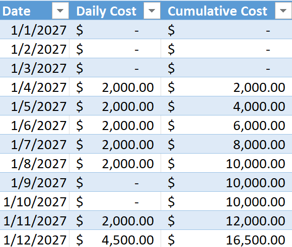
Once we have our reference data we need to create a table with all the dates from start to finish and our cost per day based from our schedule. To do this we need to create a column titled date and add the dates from the start to end (1/1/2027 to 5/31/2027 for this example). We also need a column for our daily cost and our cumulative costs.

Daily Cashflow

To get our daily cashflow we need to calculate the amount of cost per day. But we need to skip weekends and only add the amount for a task(s) that is happening on given day. To do this we use the following formula

=IF((WORKDAY([@Date]-1, 1)=[@Date])=TRUE, 
(SUMIFS(schedule[Cost per Day], 
schedule[Start Date],"<="&[@Date], 
schedule[Finish Date],">="&[@Date])), 0)

This is a long one so lets break it down. We start with an IF statement, the primary reason is we need to skip weekends. The condition for that if statement is whether the date is a week day or not (you can also add holidays). The first chunk of formula after the IF is (WORKDAY([@Date]-1, 1)=[@Date]) This uses the workday function to look at the date and returns TRUE or FALSE if its a work day, we use =TRUE after this to state that if TRUE (true being its a workday) then then use the next section of the IF statement. The next statement (SUMIFS(schedule[Cost per Day], schedule[Start Date],"<="&[@Date], schedule[Finish Date],">="&[@Date])), 0) is a SUMIFS function which will bring in the sum of all the rows in our schedule table that match our criteria. In this case we are looking for start dates that are equal to or greater than the date in our cashflow table and end dates that are equal to or less than the date in our cashflow table.

Next we need to get our cumulative cost for each date in our table. This formula will need to handle an error as the formula will reference the header. Use the following formula in the daily cashflow table

=IFERROR([@[Daily Cost]]+D3, 0)

NOTE: add this formula to the second cell down in the table and it will fill both up and down.

Vizualizing the Data

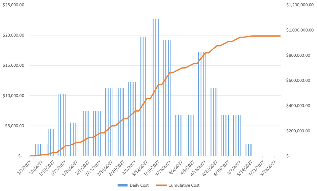
Now we want to see the data cause thats what we are really here for. Select the table and insert a bar chart and you should get something like the graph below which doesn’t help us much.

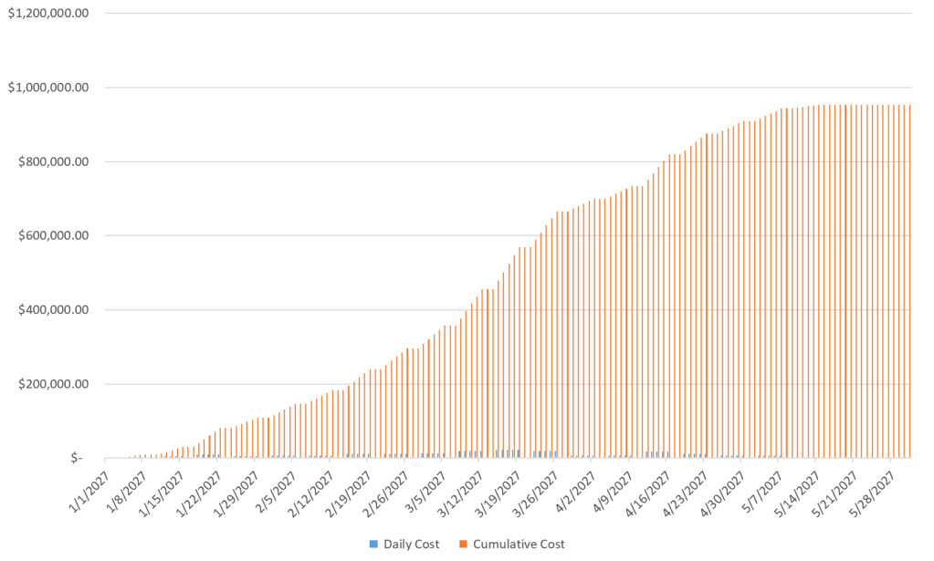
We need to do two things to make this graph readable. One we need the cumulative to be a line, two we are going to need a secondary axis. Select the chart and in Chart Design select change chart type. At the bottom choose combo chart and make sure cost is a bar and cumulative is a line and select secondary axis for cumulative.

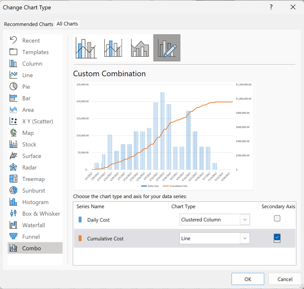
Click OK and your graph should now look like this.

But Wait Theres More

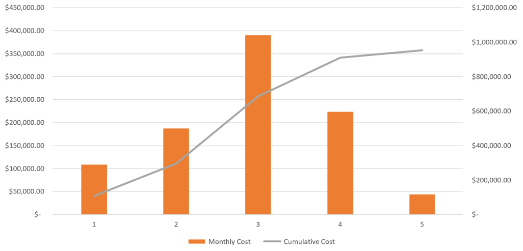
Now this is good so far but really we want to see our monthly cost as we are not usually paying bills on a project everyday and most likely your accounting team isn’t gonna care much about this graph.

We need to create a new table and have columns for months, monthly cost, and cumulative cost. We also need to create a month column on the daily cash table. In this new column we will add the formula

=MONTH([@Date])

This will return the month number for each date in the table. Next we will create a helper column off to the side of the daily table and enter the following formula

=UNIQUE(day_cash[Month])

This will give us a dynamic array with the months included in our daily table. We can then use these to populate the monthly table months column. In the monthly table we perform another sumif function but this time using the month column of the daily table.

=SUMIF(day_cash[Month],[@Month],day_cash[Daily Cost])

And we add the same cumulative cost formula into our monthly table (make sure to modify for the month table). Since we dont have multiple dates above the start date in the month column we will need to have a simple formula linking the top month into the cumulative column (doing this will overwrite the pervious formula so hit CTRL+Z once to include both formulas in this column.

Now create a graph same as before and boom you have a monthly cashflow graph.

Want and extra challenge, modify the schedule to be over a year long and do a quarterly and yearly analysis.

Now before you scratch you head and say this isnt cashflow, take the same exercise and add your revenue and your have both sides of the equation.

Resources

The excel files used in this articles can be found in the companion github repository by clicking the button below.