Monte Carlo?

This is a method of determining a range of outcomes by using random numbers to create a large set of samples. Lets say we want to know a range of costs that a given project could have. We could take our estimated cost and multiply it by a set of random factors to come up with different outcomes. Say we have $100,000 as our estimate and we multiply that by .9 we would get $90,000, and then again by 1.1 giving us $110,000. Now imagine doing that 10,000 times and we would have a large set of samples and could see a distribution of our cost projections. This in essence is a Monte Carlo Simulation.

Our Starting Data

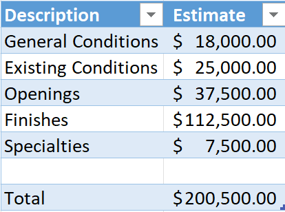
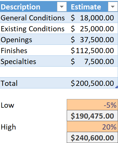
For this simple simulation we are going to use a simple estimate and we will run the simulation on the total amount only. We will have just a simple table like the one below to start with. Just outside of the table we will sum up the budget column to get our total.

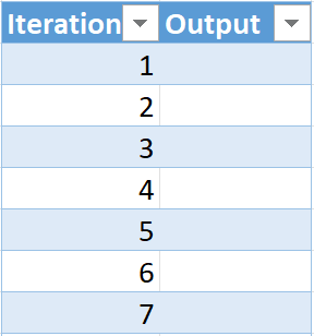
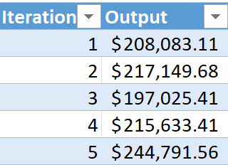
Next we need a table on a new worksheet that will hold our simulation data. This table should have two columns “Iteration” and “Output” and we can make this table 100 rows tall. In the iteration column we should have numbers 1-100.

Excel Modifications

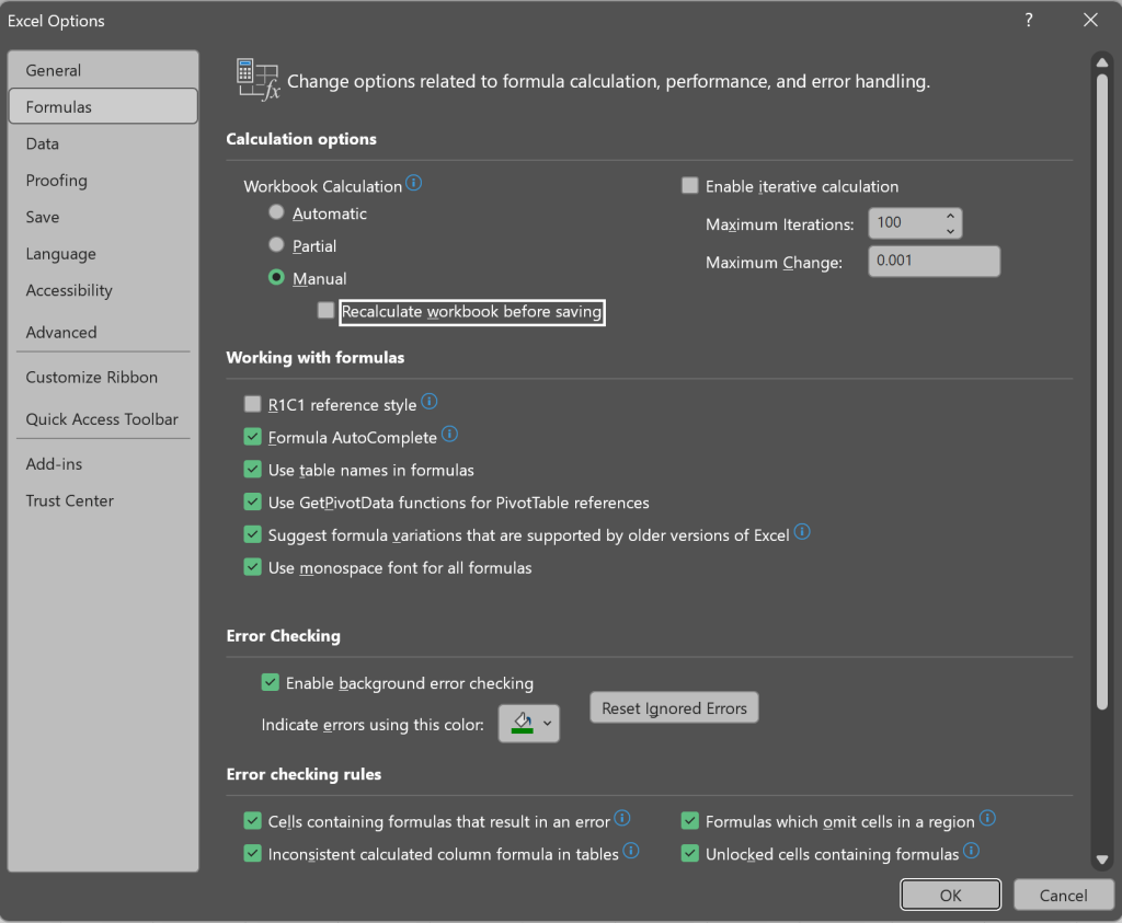
Monte Carlo Simulations are quite computationally expensive so we want to implement a couple steps to help not bog our system down. First we want to open up excel options (FILE -> OPTIONS, this is at the bottom left hand side). Inside options in the formula section you will see workbook calculations. This is most likely set to Automatic, we want to change this to Manual and uncheck the recalculate workbook before saving. This means when we write a formula the workbook will not automatically perform the calculation until we tell it to.

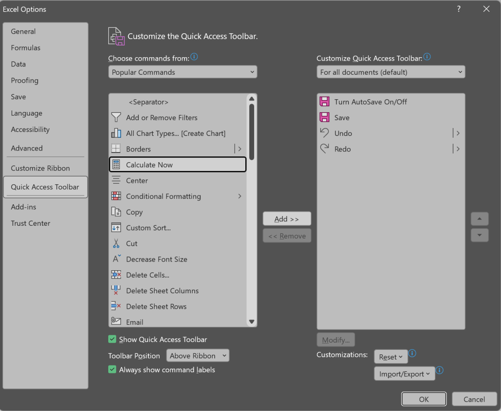
Now changing this means we need to beable to quickly tell Excel to perform calculations so on the top of the toolbar (ribbon) there is a drop down that allows you to add commands to this quick access tool bar. Youll need to click “More Commands”.

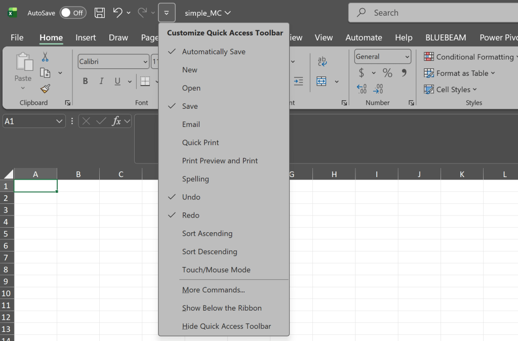
Inside the dialog box that appears select Calculate Now and click the “Add >>” button to add it to the quick access tool bar and click OK.

Simulation Formulas

Now we need to create the formulas that will allow us to perform our simulations. First we need to add an areas for us to input our range. This range is the amount of downside and upside risk we feel the project will face. This range can be determined numerous way and will not be covered here, you can run multiple estimate scenarios and determine a high, mid, and low estimate, you can apply different scenarios to each division, etc. For this example we are going to assume we have a downside risk of 20% meaning we think the highest outcome is that the project costs us 20% more than we estimated. We are also going to assume a upside risk of 5% meaning we think the best case scenario is that the project will cost us 5% less than we estimated (this will be input as a negative number as it’s less cost not more).

Let’s add a couple boxes under our total for these numbers. We can input the -5% and 20% in our boxes. Below each box create a field that takes the estimate total and multiplies it by our low and high ranges.

Performing our Simulation

Our first step is to create our output formula. Below is the formula we will put in our output column.

=NORM.INV(RAND(), AVERAGE(Simulation!$C$9,Simulation!$C$12,Simulation!$C$14), STDEV.P(Simulation!$C$9,Simulation!$C$12,Simulation!$C$14))

This formula gives us the Inverse of the normal distribution function “NORM.INV”, inside this formula we need a random number generator as this is what a Monte Carlo simulation is based on. Here we use RAND() to get our random number between 0 and 1. The next number we need is the mean and we have a couple options here so feel free to experiment, for this example we will use the average of the three estimates (the estimate, the low estimate, the high estimate), you could also use the estimate value which would impact the simulation, the average of the estimate and the high estimate as well, etc. Next for the formula we need the standard deviation where we use the STD.P() function and in here we place our three estimates (you can also experiment here as well).

We now should have a table that has our iteration number and our output which is our estimate multiplied by our random modifier. At this point we can click the calculate now button to update all our formulas.

Now we want to see our data. Lets add a histogram chart to our simulation. Click on the blank chart and click select data, go to your simulation data and select the output column only.

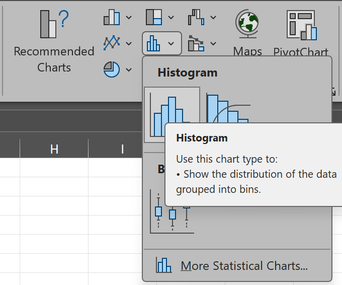
This should give you a histogram that looks like this.

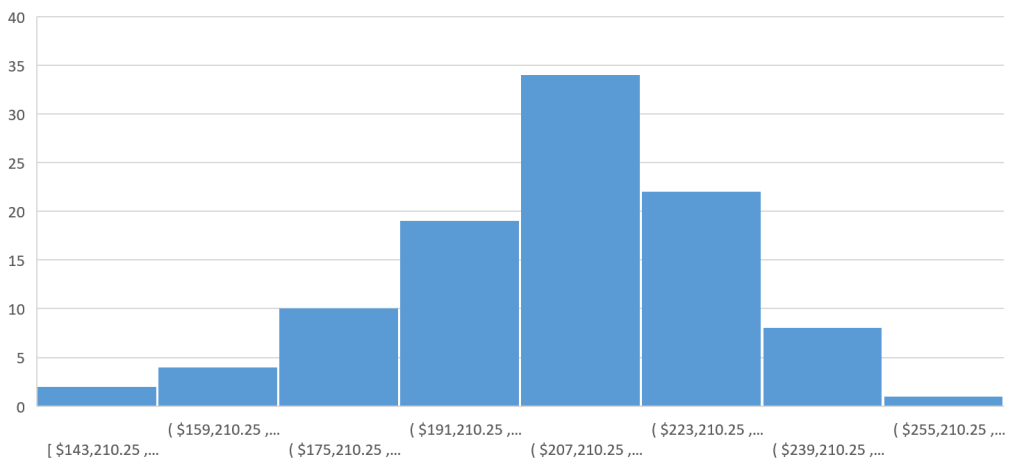
Next lets add some metrics below our graph to show the 25%, 50%, 75%, and 95% percentiles of our data. This will them us based on our simulation what 75% of our simulations will cost more that, what 50% of our simulations will cost more than, what 25% of our estimates will cost more than, and finally what 5% of our simulations will cost more than.

Once you have your percents input into your sheet add the following formula next to them. Note that the table with the simulation output data has been names “sim”.

=PERCENTILE.INC(sim[Output], F23)

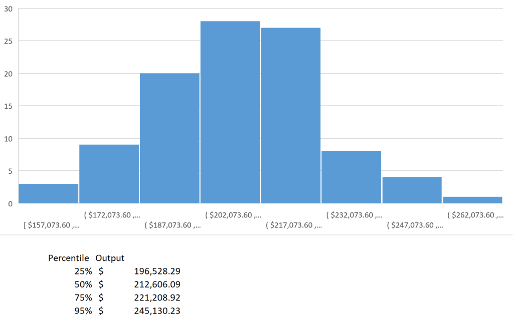
Each time you click the calculate now button on the quick access toolbar the formula will change the numbers in the RAND() function and will populate a whole new set of simulation outputs.

Now we have a basic Montel Carlo simulation built we now need one more step. Using a hundred simulations will not be enough. The method required far more simulations. So select the bottom three (this will keep the numbers going up in sequential order) cells in the iterations column and drag them down till you get 10,000 iterations (you read that right), the output column should automatically copy down as well and populate the formula. This also should automatically update the graph and the percentiles.

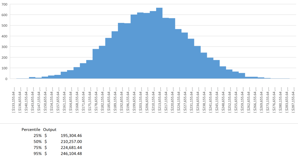
And there you have it a simple Monte Carlo simulation that runs 10,000 sims using a normal distribution based on the low and high risk measures of your estimate. It should be noted that this is only scratching the surface of Monte Carlo simulations and the complexities of measuring risk. I high recommend you continue to experiment and research how these work and their implementation.

Resources

The completed excel sheet used in this articles can be found in the companion github repository by clicking the button below.