
A what?
Yep, I am fully aware that I made that up. A multi index inflation/escalation model, a device of my own creation, well not really more of an amalgamation of ideas that were snagged from various research to create one metric to rule them all. All that aside, let’s assume for a moment that we have a basic construction project. We have concrete, wood, steel, drywall, and paint. Now each of these has its own price index tracked by the federal reserve over at uncle FRED (not familiar with FRED, there is another article HERE where we go into getting FRED data using python). This go around we are going to tap into that FRED data using R and import some indices to building our very own job specific escalation index. For this example we will keep the data and calculations as simple as possible while still building a usable system.
The Estimate
Let’s start first with a simple estimate table. We need to add a column to our estimate that is not typically in most estimates that I see. We need a column to add our FRED index label for the primary material.
Note: It should be stated that you could make this more complex and possibly more accurate by taking materials and adding multiple indices to them. Say concrete is 80% concrete and 20% steel and you could split it as such. For now we are going to just apply the primary material index.
When we arrive at the FRED website we can start searching for our materials that may have an index (you could also use the FRED excel plugin to search and bring data in that way). Once we have our indices we should place those into our estimate and we are off to the races. If you are using the data included in the repository then your estimate will look like this.
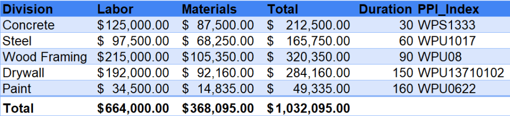
Quick note on the duration since we are escalating each item individually the duration is the total time from the start of the project. So if our steel cant happen till the concrete is done, then the duration of the concrete is added to the the steel. Assume the concrete will take 30 days and the steel starts when concrete is done and takes 30 days. Then the duration for the steel is 60 days.
A word on forecasting and trends
For this example again we are keeping things simple so we are going with a straight linear trend (using the start of our data and end of our data) using the data from a couple time periods. We will trend off the last year of data, the last 5 years of data, and the last 10 years of data. From here you can explore some more advanced forecasting methods and for more information I would highly recommend the book Forecasting: Principles & Practice which you can find as a free text book at https://otexts.com/fpp2/
Setting Up Our R Project
We start by creating a new R file (you can learn more about this in the getting started section) and we will import the required libraries.
library(dplyr)library(fredr)library(ggplot2)library(lubridate)library(tibble)library(tidyr)library(tidyverse)
For organizing our code lets add some sections where we will add our different pieces of code and allow us to expand and collapse areas making navigation a bit easier. You can skip this step if you like but I find its nice to have the option to collapse things out of the way when needed.
#### Global Var ######## Functions ######## Variables ######## Tables ######## Plots ######## Changes ####
Global Variables
If you are using the same variable names each time your could add those here. For this example we are going to add here our FRED API KEY and our date ranges and time period calculator. If you need help with this you can reference the article about using FRED data with python mentioned earlier.
fredr_set_key("YOUR API KEY HERE")
We create two variables names start and data date (data date being the end of the range). Then we create a t_per variable that calculated the amount of time between the two dates.
start_date = "2025-01-01"data_date = "2026-01-01"t_per = time_length(start_date %--% data_date, unit = "days")
If you are new to R at this point you should highlight your code from top to bottom and hit CTRL+ENTER (CMD+RETURN on mac) to execute your code and you should get some values in the IDE.

Functions
Next we will write a couple functions to pull the FRED data in and make a table for each of our indices. We will use two functions for this. The first function takes the name of a dataframe (df), the id (this is your index id), the start date, and end date that we want our data in. It takes this data and using the fredr library we installed earlier pulls in the data from FRED and makes a data frame.
fred_table <- function(df, id, start_date, end_date) { df <- fredr( series_id = id, observation_start = as.Date(start_date), observation_end = as.Date(end_date) )}
This next function takes the same inputs and also adds a multiplier and some columns to the function. We won’t worry about the multiplier but it is there as some data needs to be multiplied if you were normalizing or change the data). Inside the function it creates a dataframe using our previous function and drops some of the data that comes in from FRED that we don’t need (series _id, realtime_start, realtime_end), and adds a column for the value and multiplies that by our multiplier (which is 1 so it doesn’t change the value), and finally names the columns.
api_data_pro <- function(df, id, df_start = start_date, df_end = data_date, multiplier = 1, col1 = "col1", col2 = "col2") { df <- fred_table(df, id, df_start, df_end) df <- select(df, -c(series_id, realtime_start, realtime_end)) df$value <- df$value * multiplier colnames(df) <- c(col1, col2) return(df)}
Variables
Next we add some variables, these are where we assign the FRED index ID. These will be used to create the dataframes using the function we created earlier.
cnc_index <- "WPS1333"stl_index <- "WPU1017"lmb_index <- "WPU08"pnt_index <- "WPU0622"dry_index <- "WPU13710102"ppi_index <- "PPIACO"lab_index <- "CES2000000003"
Tables
Next we need to create tables using the indices we have chosen. Here we use the name our table (cnc), pass it to our function and inside the function we state the name of our table again (cnc), the name of the respective index variable (cnc_index), and name our columns.
cnc <- api_data_pro(cnc, cnc_index, col1 = "Date", col2 = "concrete")
We repeat this process for each of our indices.
Plots
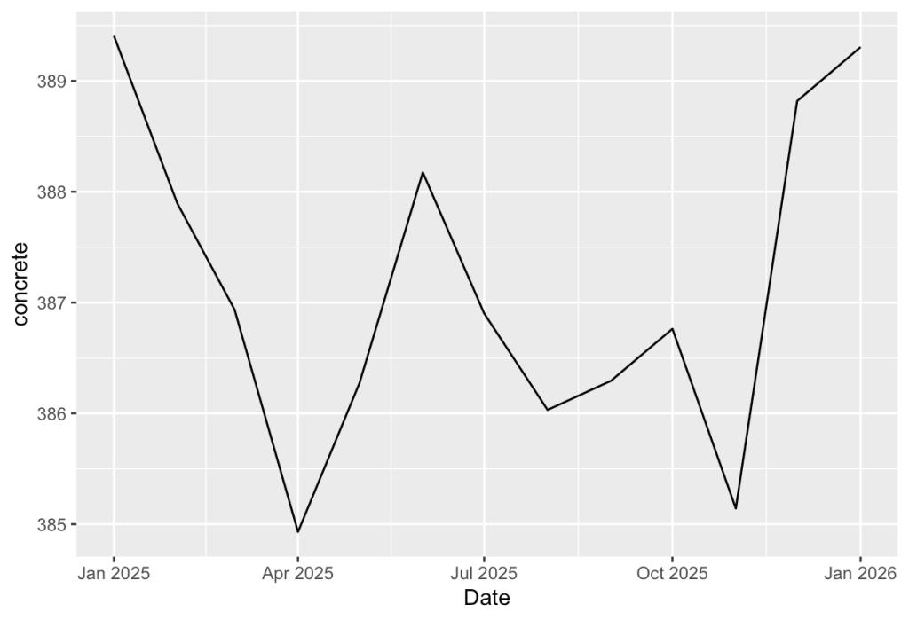
This step while optional is good idea. We want to look at the data we have brought in. Using ggplot we pass our dataframe and using the aesthic (aes()) mapping we set our x and y values for our plot. Then we add our line using geom_line().
ggplot(cnc, aes(x = Date, y = concrete)) + geom_line()
The output should look something like this. If you haven’t done so yet now would be a good time to highlight and execute your current code.
Changes
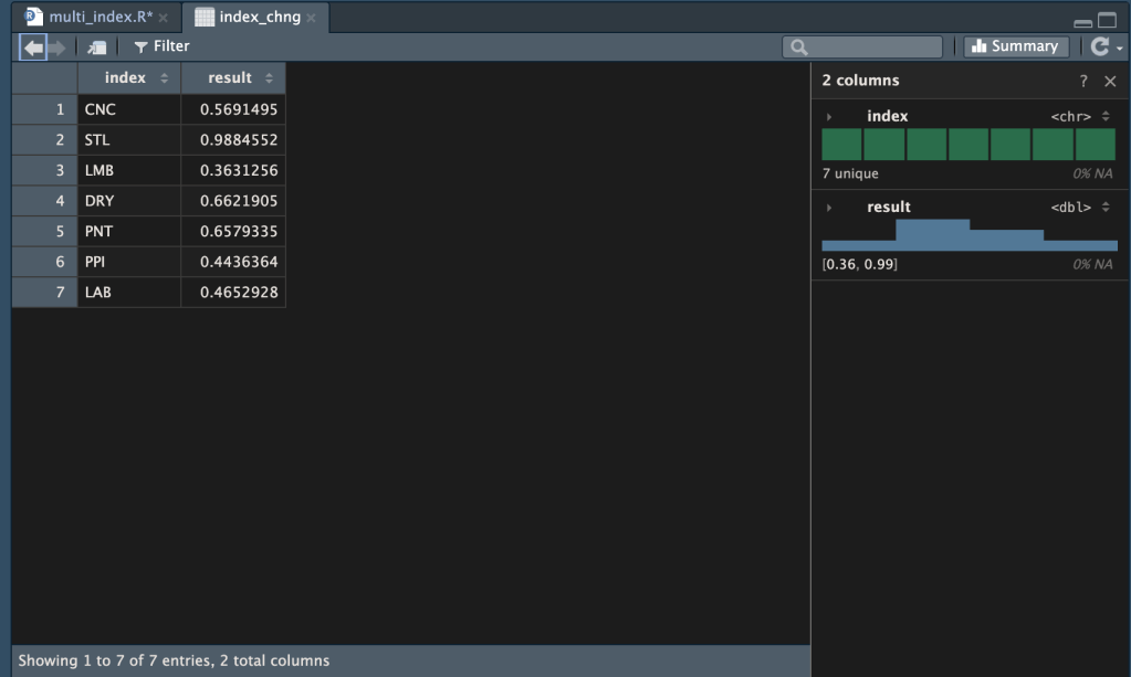
Now that we have all our data in dataframes we want to measure the change in the indices over that time period and add all those to a new dataframe we will use to adjust our estimate.
Lets break this one down, we name our new dataframe (index_chng) and we create a blank dataframe (data.frame()) inside that we name our columns (index, result) and define that one is text and one is a number.
Next we add rows for each of our indices (add_row(index = c(“CNC”, etc.) and for our result we take each index and find the last value minus the first value and divided that by the first value to get the percent change.
index_chng <- data.frame(index = character(0), result = numeric(0))index_chng <- index_chng %>% add_row(index = c("CNC", "STL", "LMB", "DRY", "PNT", "PPI", "LAB"), result = c( cnc %>% summarise(result = ((last(concrete) - first(concrete)) / first(concrete))) %>% pull(result), stl %>% summarise(result = ((last(steel) - first(steel)) / first(steel))) %>% pull(result), lmb %>% summarise(result = ((last(lumber) - first(lumber)) / first(lumber))) %>% pull(result), dry %>% summarise(result = ((last(drywall) - first(drywall)) / first(drywall))) %>% pull(result), pnt %>% summarise(result = ((last(paint) - first(paint)) / first(paint))) %>% pull(result), ppi %>% summarise(result = ((last(ppi) - first(ppi)) / first(ppi))) %>% pull(result), lab %>% summarise(result = ((last(lab) - first(lab)) / first(lab))) %>% pull(result) ) )
This should give us a new dataframe with our results which is our percentage change from the start to the end of the period.
Finally we need to export this data to a CSV so we can take it and update our estimate.
write.csv(index_chng, "index_chng.csv")
Updating the Estimate
Lets add a few columns to our simple estimate table. Material Index Change where we can add the data from our code, Material Increase where we can calculate the change, Labor Index Change, Labor Increase, and lastly an Escalated column where we can add the increase to the base estimate. We also added a PPI1 value to our dataframe so we can compare that to the escalation our other indices produce.
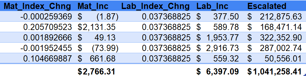
The formula in our increase column could be a number of things based on how you want to calculate the increase but the formula used in the example is as follows. The number “365”2 in the formula below is the number we got in our code in the t_per variable, as we change the start and data dates of our code this number will change.
=[@Estimate]*((1+[@[Index_Chng]])^([@Duration]/365)-1)
From there you need to do the same thing for the labor index to find the increase to the labor. Once this is done you can simply add the numbers (labor, material, material increase, and labor increase) together and you will have your escalated estimate.
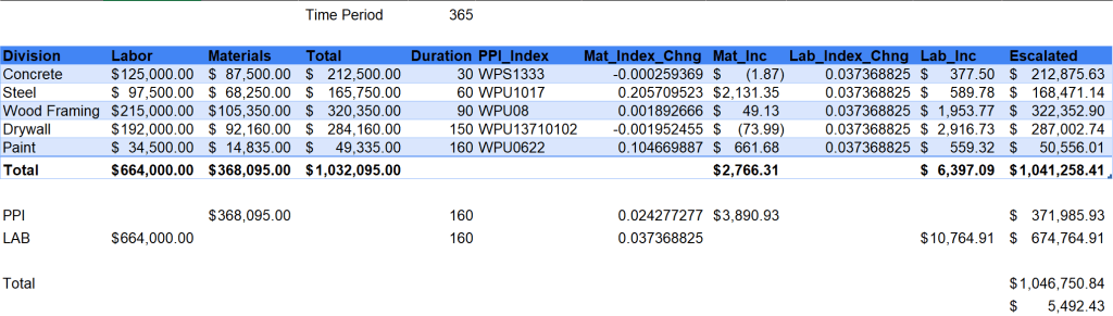
Now that we have that done lets check out a 5 & 10 year data range and see how that impacts our results.

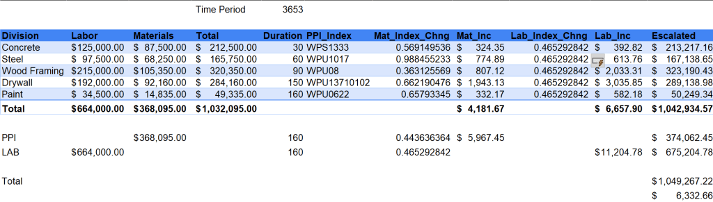
From here you can explore larger datasets, integrate this into excel or your estimating system better, make the overall code simpler and more efficient, etc. Remember your creativity is the only barrier in what you can create.
Resources
The code and notebooks used in this articles can be found in the companion github repository by clicking the button below.

